Sugihara’s Circle/Square Optical Illusion

[Update: Check out my second post in which I provide a template so you can make your own Sugihara circle/square object out of paper.]

Kokichi Sugihara created a video called Ambiguous Optical Illusion: Rectangles and Circles. In it he shows a variety of 3-dimensional objects that look like one shape when viewed from the front but look like a different shape in the mirror behind it.

In this blog post we show how he achieved the effect. For simplicity, we will show how he made a shape that looks like a circular cylinder from the front and a square cylinder in the mirror.

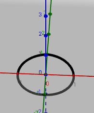
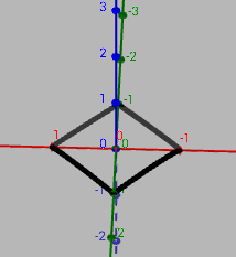
The following applet shows our final product (clicking the image links to the GeoGebra applet). It is a closed curve that represents the top rim of Sugihara’s shape. You can rotate the axes with your mouse. If you view the coordinate system with the positive green and blue axes lined up (1 with 1, 2 with 2, and so on), the curve will look like the unit circle in the green-red plane. If you drag the image so that the positive blue axis lines up with the negative green axis (1 with -1, 2 with -2, and so on), it will look like you are viewing a square (oriented as a diamond) in the green-red plane.

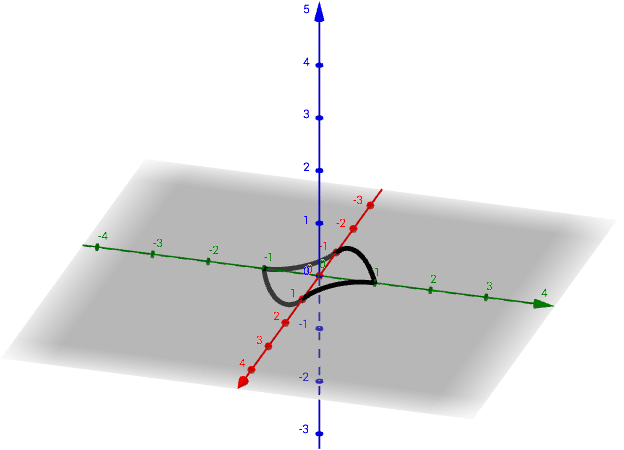
Here are screenshots showing the two views.

circle square

How does it work? It is all about perspective.

To set this up mathematically, we imagine two viewers in 3-dimensional space. One viewer is at ${P(0,a,a)}$ and the other is at ${Q(0,-a,a)}$ (in the video this second viewer is you, in the mirror). They are looking down on a curve ${\mathbf{r}(t).}$ However, from their vantage points it looks like they are seeing two different curves in the ${xy}$ -plane: ${\langle u, f(u),0\rangle}$ and ${\langle u, g(u),0\rangle,}$ respectively.

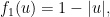
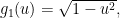
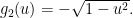
In our example the two observed curves are the unit circle and the square passing through the points ${(\pm 1, \pm 1, 0)}$ , as shown in the ${xy}$ -plane below. We will have to break each of these shapes into two different curves, so we’ll have ${f_{1}(u)=1-|u|,}$ ${f_{2}(u)=|u|-1,}$ ${g_{1}(u)=\sqrt{1-u^{2}},}$ and ${g_{2}(u)=-\sqrt{1-u^{2}}.}$ Also, we could choose ${a}$ to be some suitably large number greater than 1, but in fact, as we will see, taking the limit as ${a}$ tends to infinity produces a lovely final expression. For now we will continue to work in generalities and will wait to insert these specifics later.

xyplane

Our aim is now to define ${\mathbf{r}(t).}$ Let’s fix ${t}$ , and let ${A(t,f(t),0)}$ and ${B(t,g(t),0)}$ be two points on the curves in the ${xy}$ -plane. In order for the person at ${P}$ to view her shape, ${\mathbf{r}(t)}$ must lie on the line ${AP}$ (see figure below). Likewise, for the person at ${Q}$ to see his shape, ${\mathbf{r}(t)}$ must lie on the line ${BQ.}$ Thus, ${\mathbf{r}(t)}$ must be the point of intersection of lines ${AP}$ and ${BQ.}$ (We know that the lines are not skew because they lie in the plane containing the points ${P,}$ ${Q,}$ and ${(t,0,0),}$ and for appropriate choices of ${f,}$ ${g,}$ and ${a}$ the lines intersect and the point of intersection is below ${z=a.)}$

xyzpic

It is straightforward to show that ${\mathbf{r}_{AP}(s)=\langle ts, (f(t)-a)s+a, -as+a\rangle}$ is a parametrization of the line ${AP}$ and ${\mathbf{r}_{BQ}(s)=\langle ts, (g(t)+a)s-a, -as+a\rangle}$ is a parametrization of ${BQ.}$ A little algebra shows shows that their point of intersection is

$\displaystyle \left(\frac{2at}{g(t)-f(t)+2a},\frac{af(t)+ag(t)}{g(t)-f(t)+2a},\frac{ag(t)-af(t)}{g(t)-f(t)+2a}\right),$

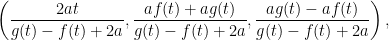
and thus our desired curve is

$\displaystyle \mathbf{r}(t)=\tfrac{a}{g(t)-f(t)+2a}\cdot\langle2t,f(t)+g(t),g(t)-f(t)\rangle.$

Because ${a}$ is a large value, we can take the limit as ${a}$ goes to infinity. This yields the elegant expression

$\displaystyle \mathbf{r}(t)=\langle t,\tfrac12(f(t)+g(t)),\tfrac12(g(t)-f(t))\rangle.$

We may now plug in our functions. The portion of our curve with nonnegative ${y}$ -coordinates is given by

$\displaystyle \mathbf{r}_{1}(t)=\langle t,\tfrac12(1-|t|+\sqrt{1-t^{2}}),\tfrac12(\sqrt{1-t^{2}}+|t|-1)\rangle$

for ${-1\le t\le 1,}$ and the other half by

$\displaystyle \mathbf{r}_{2}(t)=\langle t,\tfrac12(|t|-1-\sqrt{1-t^{2}}),(1-\sqrt{1-t^{2}}-|t|)\rangle$

for ${-1\le t\le 1.}$ This is the curve shown in the applet.

[Update: See the comment by Joshua and my reply for a simpler way of obtaining the parametrization.]

8 Comments

Pingback: La quadratura del cerchio [Pillole] | backup del Post
Pingback: L’illusione della quadratura del cerchio [Pillole] | backup del Post
John Baez says:

July 6, 2016 at 4:10 am

Great! I understand it now.
Pingback: Make a Sugihara Circle/Square Optical Illusion Out of Paper | Division by Zero
Joshua says:

July 6, 2016 at 9:02 pm

This was very helpful. With your derivation as the inspiration, I think there is another nice way to see the required curve.

Consider lines between an observer at (0, a, a) and points on the plane y = – z. As a gets larger, these lines get closer to being parallel and perpendicular to the plane. This means that the observer from that position will perceive points in space closer and closer to their perpendicular projections onto that plane (a, b, c) -> (a, b-c, c-b).

Similarly, for the observer at (0, -a, a) and the plane y = z, with the projection (a, b, c) -> (a, b+c, b+c).
1. Dave Richeson says:
  
  July 7, 2016 at 11:35 am
  
  Joshua—Thanks for your comment. That’s a great way to think about it. Another way to think about it (which is essentially the same as your way) is to make the simplifying assumption that the vector from a point on the plane curve to the viewer’s eye is parallel to $\langle 0,1,1\rangle$ (and $\langle 0,-1,1\rangle$ for the other viewer). Then the line from the points on the curves to the viewers’ eyes are 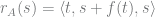$r_A(s)=\langle t,s+f(t),s\rangle$ and $r_B(s)=\langle t,-s+g(t),s\rangle.$ It is easy to find the point of intersection of those lines.
nosedog says:

July 6, 2016 at 9:32 pm

That is so awesome. Thanks for this great exposition.
Pingback: Wild Maths, Ambiguous Cylinders, and 228 Women | Math Munch